Resonance does not occur only in the triangular case, when the circulation (= flux) ratio is 1. It is known in the stationary case (I believe, due to Igor Loutsenko and Oksana Yermolayeva) that there is also a hierarchy of resonances for the circulation ratio 1:2. This is also true in the translating-vortices case, but is significantly more complicated. Let’s illustrate this in the simplest non-trivial case, using a few lines of Mathematica code:
P[z_] := z/2 + z^3 + aQ[z_] := 3/4 + 10 z^4 + (9 z^5)/2 + z^6 - (3 a)/8 + a^2 + 2 z^3 (6 + a) + z^2 (7 + (9 a)/2) + 1/4 z (6 + 13 a)
These two polynomials satisfy the Tkachenko equation:
S[P_, Q_, z_] := D[P, {z, 2}]Q - 2\[Lambda] D[P, z] D[Q, z] + \[Lambda]^2 D[Q, {z, 2}] P + 2 (D[P, z]*Q - \[Lambda] P D[Q, z]);\[Lambda] = 1/2;(*circulation ratio*)S[P[z], Q[z], z] // Simplify(*you should get 0*)
Now define Weierstrass data. The integrals are mostly explicit, thanks to Tkachenko.
dh[z_] := 1 + P'[z]/P[z] - \[Lambda] Q'[z]/Q[z]G[z_] := \[Rho] dh[z]DH[z_] = Integrate[dh[z], z];GDH[z_] := \[Rho] (z - (P'[z]/P[z] + \[Lambda]^2 Q'[z]/Q[z]))G1DH[z_] := z/\[Rho]f[z_] := Re[{(G1DH[z] - GDH[z])/2, I (G1DH[z] + GDH[z])/2, DH[z]}]
It’s time to choose parameters: a is an arbitrary complex number, and Rho determines the tilt of the planar end, thanks to López-Ros.
a = .5 I;(*choose your own*)\[Rho] = .1;(*very little tilt is looking better*)
To get a surface image, we triangulate a punctured disk. The holes in the image are enlarged to make them better visible.
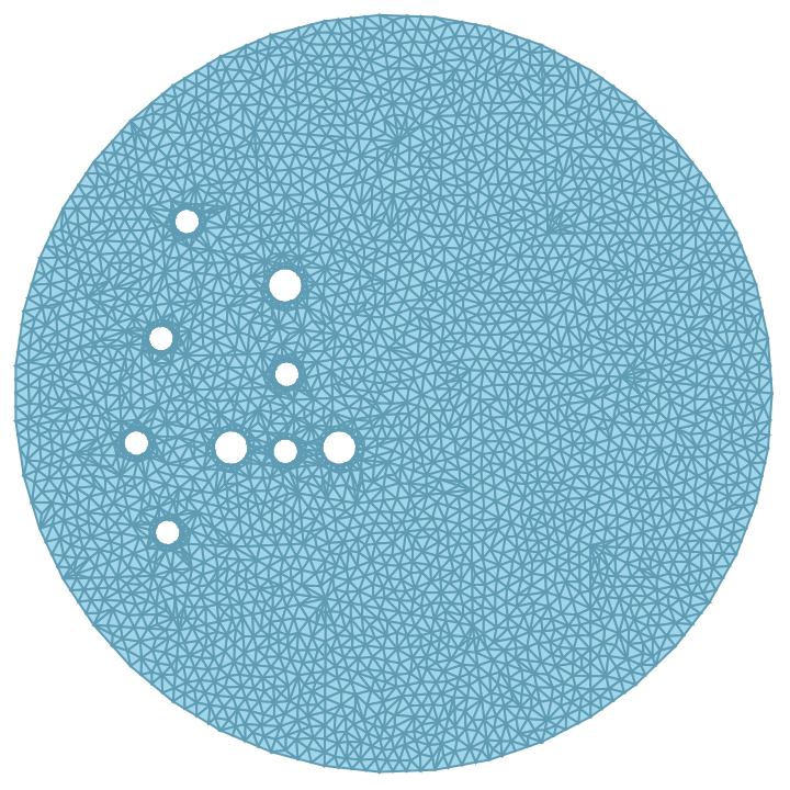
punctures = Join[z /. NSolve[P[z] == 0, z], z /. NSolve[Q[z] == 0, z]];outerDisk = Disk[{1, 0}, 3.5];holes = RegionUnion @@ MapThread[ Disk[#1, #2] &, {ReIm[punctures], Join[.02 Array[1 &, Exponent[P[z], z]], .015 Array[1 &, Exponent[Q[z], z]]]}];hollowRegion = RegionDifference[outerDisk, holes];triangulation = DiscretizeRegion[hollowRegion, MaxCellMeasure -> 0.01]vertices = Apply[Complex, MeshCoordinates[triangulation], 1];

Finally, we can render the minimal surface version of the vortex configuration.
StereographicProjection[ z_] := {(2*Re[z])/(1 + Abs[z]^2), (2*Im[z])/(1 + Abs[z]^2), 1 - 2/(1 + Abs[z]^2)};coords = Map[f, vertices];normals = Map[StereographicProjection[G[#]] &, vertices];Show[Graphics3D[{EdgeForm[], g1 = GraphicsComplex[coords, MeshCells[triangulation, 2], VertexNormals -> normals]}], Boxed -> False]
The resonance can be made visible by varying the parameter a:
You can use the same lines of code to render vortex/minimal surface configuration in the (6,12) case, except that now you have two parameters:
P[z_] := z^6 + (5 z^4)/2 + s z^3 - (5 z^2)/4 + u z - s^2/5 - 35/24;Q[z_] := z^12 + 9 z^11 + (173 z^10)/4 + (1065/8 + 2 s) z^9 + (4425/16 + (27 s)/2) z^8 + (1575/4 + (91 s)/2 + 2 u) z^7 + (1165/3 + (375 s)/4 + (3 s^2)/5 + (21 u)/2) z^6 + (4335/16 + (1015 s)/8 + (27 s^2)/10 + (101 u)/4) z^5 + (9575/96 + 120 s + (23 s^2)/4 + 30 u + 2 s u) z^4 + (-(325/8) + (1595 s)/24 + (21 s^2)/2 - (2 s^3)/5 + (25 u)/2 + 6 s u) z^3 + (2725/192 - (75 s)/8 + (121 s^2)/8 - (9 s^3)/10 + (27 s u)/4 + u^2) z^2 + (6625/128 - (165 s)/16 + (129 s^2)/16 - (9 s^3)/20 + (5 u)/6 + (45 s u)/8 - (2 s^2 u)/5 + (3 u^2)/2) z + 60025/2304 - (105 s)/32 + (371 s^2)/96 - (9 s^3)/20 + s^4/25 + (5 u)/8 + (45 s u)/16 - (3 s^2 u)/10 + (3 u^2)/4;
And this is only the beginning. We will report soon.


